18~24 February 2013 (week 5 )

Title Of Activity 

-Project Progress :

 -Saving a data .

-Adding a Button That stores data when clicked .

Objectives

-To store information about the data a VI generates.

-Click the button to store the data.

-Run the program and see the storing information of the progress.

Content/Procedure

-To store information about the data a VI generates, use the Write To Measurement File Express VI.

-Complete the following steps to build a VI that saves peak-to-peak values and other information to a LabVIEW data file.

1. Search for the Write To Measurement File Express VI and add it to the block diagram below and to the right of the Amplitude and Level Measurements Express VI.

The Configure Write To Measurement File dialog box appears.The Filename text box displays the full path to the output file,test.lvm. A .lvm file is a tab-delimited text measurement file you

can open with a spreadsheet application or a text-editing application.LabVIEW saves data with up to six digits of precision in a .lvm file. LabVIEW saves the .lvm file in the default LabVIEW Data

directory. LabVIEW installs the LabVIEW Data directory in thedefault file directory of the operating system.When you want to view the data, use the file path displayed in the Filename text box to access the test.lvm file.

2. In the Configure Write to Measurement File dialog box, locate theIf a file already exists section and select the Append to file option to write all the data to the test.lvm file without erasing any existing

data in the file.

3. In the Segment Headers section, select the One header only optionto create only one header in the file to which LabVIEW writes the data.

4. Enter the following text in the File Description text box: Sample of peak to peak values. LabVIEW appends the text you enter in this text box to the header of the file.

5. Click the OK button to save the current configuration and close the Configure Write To Measurement File dialog box.

-Saving Data To A File 

-When you run the VI, LabVIEW saves the data to the test.lvm file. Complete the following steps to generate the test.lvm file:

1. On the block diagram, wire the Peak to Peak output of the Amplitude and Level Measurements Express VI to the Signals input of the Write To Measurement File Express VI.

2. Select File»Save As and save the VI as Save Data.vi in an easily accessible location.

3. Display the front panel and run the VI.

4. Click the front panel STOP button.

5. To view the data you saved, open the test.lvm file in the LabVIEW Data directory with a spreadsheet or text-editing application. 

The file has a header that contains information about the Express VI.

6. Close the file after you finish looking at it and return to the Save Data VI.

-Adding a Button That Stores Data When Clicked

-If you want to store only certain data points, you can configure the Write To Measurement File Express VI to save peak-to-peak values only when a user clicks a button.

Complete the following steps to add a button to the VI and configure how the button responds when a user clicks it.

1. Display the front panel and search the Controls palette for a rocker button. Select one of the rocker buttons and place it to the right of the waveform graphs.

2. Right-click the rocker button and select Properties from the shortcut menu to display the Boolean Properties dialog box.

3. Change the label of the button to Write to File.

4. On the Operation page of the Boolean Properties dialog box, select Latch when pressed from the Button behavior list.

Use the Operation page to specify how a button behaves when a user clicks it. To see how the button reacts to a click, click the button in the Preview Selected Behavior section.

5. Click the OK button to save the current configuration and close

the Boolean Properties dialog box.

6. Save the VI.

-Viewing Saved Data

-Complete the following steps to view the data that you save to the Selected Samples.lvm file.

1. Display the front panel and run the VI. Click the Write to File button several times.

2. Click the STOP button.

3. Open the Selected Samples.lvm file with a spreadsheet or text-editing application. The Selected Samples.lvm file differs from the test.lvm file. test.lvm recorded all the data generated by the Save Data VI, whereas Selected Samples.lvm recorded data only when you

clicked the Write to File button.

4. Close the file after you finish looking at it.

5. Save and close the VI.

                      

                           Figure 1 : block diagram of save data .

                            Figure 2 : front panel of save data .

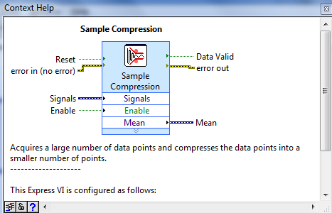
                            Figure 3 : context help box of Write To Measurement File .

Result&Analysis 

-The write to measurement file express VI saves data A VI generates and analysis to a .1vm, tdm, or , tdms measurement file .

- Get to know how to save the data and view it as well after the storing operation is completed .

  

25 February~3 March 2013 (week 6 )

Title Of Activity

-Project Progress 

  -Modifying a signal .

  -Customizing a user interface from the block diagram .

  -Controlling the speed of execution.

  -Using a table to display the data .

  -Using the cursor to get the exact value that we want .

Objectives

-Learn how to build the block diagram to modifies the signal .

-To customize a user interface from the block diagram .

-To control the speed of execution.

Content/Procedure

-Customizing a user interface from the block diagram :

-In the previous exercises, you added controls and indicators to the front panel using the Controls palette. You also can create controls and indicators from the block diagram.

-Complete the following steps to create controls and indicators from the

block diagram.

1. On the block diagram, right-click the Mean output of the Sample Compression Express VI and select Create»Numeric Indicator from the shortcut menu to create a numeric indicator. A Mean indicator,

shown at left, appears on the block diagram.

2. Right-click the Mean output of the Sample Compression Express VI and select Insert Input/Output from the shortcut menu to insert the Enable input.  In previous exercises, you learned to add inputs and outputs by expanding the Express VI using the down arrows. Using the shortcut menu is a different way to display and select the inputs and outputs of an Express VI.

3. Right-click the Enable input and select Create»Control from the shortcut menu to create a switch. A Boolean control, shown at left, appears on the block diagram.  Control terminals have a thicker border than indicator terminals. Also, an arrow appears on the right of the terminal if the terminal is a control,

and an arrow appears on the left of the terminal if the terminal is an indicator.

4. Right-click the wire that connects the Sine output of the Simulate Signal Express VI to the Signals input of the Sample Compression Express VI and select Create»Graph Indicator from the shortcut

menu.

5. Use the Wiring tool to wire the Mean output of the Sample

Compression Express VI to the Sine graph indicator. 

The Merge Signals function appears.

-Controlling the speed of execution:

-To plot the points on the waveform graph more slowly, you can add a time delay to the block diagram.

-Complete the following steps to control the speed at which the VI runs:

1. On the block diagram, search for the Time Delay Express VI, shown at  left, on the Functions palette and place it inside the While Loop. You can use the Time Delay Express VI to control the execution rate  of the VI.

2. Enter 0.25 in the Time delay (seconds) text box.  This time delay specifies how fast the loop runs. With a 0.25 second time delay, the loop iterates once every quarter of a second.

3. Click the OK button to save the current configuration and close the Configure Time Delay dialog box.

4. Display the front panel and run the VI.

5. Click the Enable switch and examine the change on the graph. If the Enable switch is on, the graph displays the reduced signal. If the Enable switch is off, the graph does not display the reduced signal.

6. Click the STOP button to stop the VI.

-Using a table to display the data :.

-Complete the following steps to display a collection of mean values in a front panel table :

1. Display the front panel.

2. On the Controls palette search for the Express Table indicator and  add it to the right of the waveform graph.

3. Display the block diagram. LabVIEW wired the Table terminal to the Build Table Express VI.

4. If the Build Table Express VI and the Table terminal are not selected already, click an open area on the block diagram to the left of the Build Table Express VI and the Table terminal. Drag the cursor diagonally until the selection rectangle encloses the Build Table Express VI and the Table terminal, shown at left.  A moving dashed outline, called a marquee, highlights the Build Table Express VI, the Table terminal, and the wire joining the two.

                           Figure 1 : Block diagram of modifying a signal an controlling the speed of execution.

                             Figure 2 :Front panel modifying a signal an controlling the speed of execution.

-In this progress i have used the not or gate as its described in figure 3 :

Result&Analysis 

-In this progress i have used the decoration to decorate the front panel to give a nice background of the  front panel , if you are willing to do the same , here is the step :

1-From the front panel go to the view , then select tools palette to control the coloring and so on .

2-From the function palette go to modern then select decoration, from there got many choices of choosing the shape that we want to use such as : thick lower box or lowered rounded box , flat circle , raised circle , ETC. 

-Therefore, the using of not or gate computes the logical nor of the inputs as we can see at the signal once we run it .

4 ~ 17 February 2013 (week 4 )

Title Of Activity

-Project Progress

 Using filtering to filter the signal .

 

Objectives

-The filter Express VI processes signals through filters and window. We use the filtering signal to remove the noise from a signal .

-Get to know what type of filter that am i going to use in the project , and what is the type of filters ?

-Compare and absorb the differences in both signal ( filtered , unfiltered ) . 

Content /Procedure 

-The types of filters are many such as Specifies the following types of filters to use: lowpass, highpass, bandpass, bandstop, or smoothing. The default is Lowpass.

-Filtering specification : Contains the following options:

• Cutoff Frequency (Hz)—Specifies the cutoff frequency of the filter. This option is available only when you select Lowpass or Highpass from the Filtering Type pull-down menu. The default is 100.
• Low cutoff frequency (Hz)—Specifies the low cutoff frequency of the filter. Low cutoff frequency (Hz) must be less than High cutoff frequency (Hz) and observe the Nyquist criterion. The default is 100. This option is available only when you select Bandpass or Bandstop from the Filtering Type pull-down menu.
• High cutoff frequency (Hz)—Specifies the high cutoff frequency of the filter. High cutoff frequency (Hz) must be greater than Low cutoff frequency (Hz) and observe the Nyquist criterion. The default is 400. This option is available only when you select Bandpass or Bandstop from the Filtering Type pull-down menu.
• Finite impulse response (FIR) filter—Creates an FIR filter, which depends only on the current and past inputs. Because the filter does not depend on past outputs, the impulse response decays to zero in a finite amount of time. Because FIR filters return a linear phase response, use FIR filters for applications that require linear phase responses.
• Taps—Specifies the total number of FIR coefficients, which must be greater than zero. The default is 29. This option is available only when you select the Finite impulse response (FIR) filter option. Increasing the value of Taps causes the transition between the passband and the stopband to become steeper. However, as the value of Taps increases, the processing speed becomes slower.
• Infinite impulse response (IIR) filter—Creates an IIR filter that is a digital filter with impulse responses that can theoretically be infinite in length or duration.
• Topology—Determines the design type of the filter. You can create either a Butterworth, Chebyshev, Inverse Chebyshev, Elliptic, or Bessel filter design. This option is available only when you select the Infinite impulse response (IIR) filter option. The default is Butterworth.
• Order—Order of the IIR filter, which must be greater than zero. This option is available only when you select the Infinite impulse response (IIR) filter option. The default is 3. Increasing the value of Order causes the transition between the passband and the stopband to become steeper. However, as the value of Order increases, the processing speed becomes slower, and the number of distorted points at the start of the signal increases.
• Moving average—Yields forward-only (FIR) coefficients. This option is available only when you select Smoothing from the Filtering Type pull-down menu.
• Rectangular—Specifies that all samples in the moving-average window are weighted equally in computing each smoothed output sample. This option is available only when you select Smoothing from the Filtering Type pull-down menu and the Moving average option.
• Triangular—Specifies that the moving weighting window applied to the samples is triangular with the peak centered in the middle of the window, ramping down symmetrically on both sides of the center sample. This option is available only when you select Smoothing from the Filtering Type pull-down menu and the Moving average option.
• Half-width of moving average—Specifies the half-width of the moving-average window in samples. The default is 1. For a half-width of moving average of M, the full width of the moving-average window is N = 1 + 2M samples. Therefore, the full width N is always an odd number of samples. This option is available only when you select Smoothing from the Filtering Type pull-down menu and the Moving average option.
• Exponential—Yields first-order IIR coefficients. This option is available only when you select Smoothing from the Filtering Type pull-down menu.
• Time constant of exponential average—Specifies the time constant of the exponential-weighting filter in seconds. The default is 0.001. This option is available only when you select Smoothing from the Filtering Type pull-down menu and the Exponential option.

                            Figure 1 : context help of filter .

                            Figure 2 : block diagram of filtering .

                              

                            Figure 3 : front panel of filtering .

 Result & Analysis 

-From the filtered signal  we can remove the noise from the signal .-Get to know the types of  filtered that i'm going to use which is low pass filter , Infinite impulse response (IIR) filter—Creates an IIR filter that is a digital filter with impulse responses that can theoretically be infinite in length or duration .
       

 

28~3 February 2013 (week 3)

Title of Activity 

-Project progress 

  Using a table to display data .

Objectives 

-Build the table to display data .

-Reduces the number of samples in the signal .

Content /Procedure 

-In the following progress i have opened and added structures and express VIs to the block diagram to build a new VI. and i have build a VI that generates a signal , reduces the number of samples in the signal , and display the resulting data in a front panel table .

-In this exercise as well i have learned to open the context help window that display basic information about LabVIEW objects when you move the cursor over each objects.Objects will context help information include VIs. Function , structures and palettes, dialog box components, and so on.

-Displaying data in a table : the table indicator displays generated data. Use the build table Express VI to build a table of generated data of means values.

                          Figure 1 : block diagram to display data of the mean values 

                           Figure 2 : front panel to display the data of the means value using table .

                            Figure 3 : Context help showing the description of sample Compression .

  

                        

                         

Result&Analysis 

-From this exercise or progress of the final year project i could manage to display the values of means in a table by buiding the proper bock diagram and get the proper signal , means values from that signal .

-From this exercise or progress as well i learned if you want to get any explanation or function of any of the tools you just have to refer back to context help , context help provide you anything that you might need in the progress of dealing with LabVIEW and make it short term to understand the concept.

    

                            

Sunday, 27 January 2013

20 ~ 26 January 2013 (Week 2)

 Title of Activity

-Doing the exercise for getting started with LABVIEW in order to get the concept from the software chapter by chapter .

Objective: 

-To understand what is LABVIEW and what is the procedure for it .

-Analyse the signal of each part and construct the block diagram for it to get the signal .

 Content/Procedure:

-Acquiring a signal .

-Wile loop .

-Adding a knob to the front panel to control the amplitude .

 

-The front panel controls simulate the input on a physical instruments and supply data to the block diagram of the VI.Many physical instruments have knobs you can turn to change an input value .

-For the block diagram as shown below is showing the simulate signal wired up with wave graph to get the fully signal , by controlling by the knobs you can turn to change the input value and amplitude as well .

-the while loop , the terminal inside the loop are representation of front panel controls and indicators.Terminal are entry and exits ports that exchange information between the front panel and block diagram .

Result & Analysis

-As a result for this week to make sure that we can get the signal of acquiring signal through some of the controls such as knobs to turn the input value and the amplitude as well , and adding while loop to the block diagram .

-As analysis , to get the concept of building a virtual instruments .